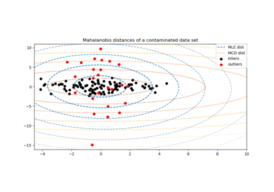
穩健 vs 經驗共變異數估計#

通常的共變異數最大概似估計對於資料集中離群值的存在非常敏感。在這種情況下，最好使用共變異數的穩健估計器，以保證估計對資料集中「錯誤」的觀測值具有抵抗力。[1], [2]

最小共變異數行列式估計器#

最小共變異數行列式估計器是一個穩健、高崩潰點 (即它可用於估計高度污染資料集的共變異數矩陣，最多達到 \(\frac{n_\text{samples} - n_\text{features}-1}{2}\) 個離群值) 的共變異數估計器。其想法是找到 \(\frac{n_\text{samples} + n_\text{features}+1}{2}\) 個觀測值，這些觀測值的經驗共變異數具有最小的行列式，從而產生一個「純」的觀測值子集，從中計算位置和共變異數的標準估計。在進行一個旨在補償估計值僅從初始資料的一部分學習的事實的校正步驟之後，我們最終得到了資料集位置和共變異數的穩健估計。

最小共變異數行列式估計器 (MCD) 是由 P.J.Rousseuw 在 [3] 中提出的。

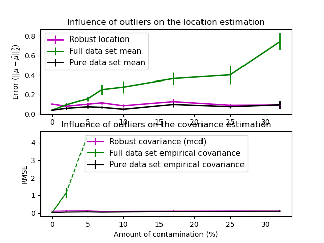
評估#

在此範例中，我們比較了在污染的高斯分佈資料集上使用各種型別的位置和共變異數估計時所發生的估計錯誤

完整資料集的平均值和經驗共變異數，一旦資料集中存在離群值就會失效
穩健的 MCD，當 \(n_\text{samples} > 5n_\text{features}\) 時具有較低的錯誤
已知是好的觀測值的平均值和經驗共變異數。這可以被認為是「完美」的 MCD 估計，因此可以透過與這種情況進行比較來信任我們的實作。

參考文獻#

Influence of outliers on the location estimation, Influence of outliers on the covariance estimation

# Authors: The scikit-learn developers
# SPDX-License-Identifier: BSD-3-Clause

import matplotlib.font_manager
import matplotlib.pyplot as plt
import numpy as np

from sklearn.covariance import EmpiricalCovariance, MinCovDet

# example settings
n_samples = 80
n_features = 5
repeat = 10

range_n_outliers = np.concatenate(
    (
        np.linspace(0, n_samples / 8, 5),
        np.linspace(n_samples / 8, n_samples / 2, 5)[1:-1],
    )
).astype(int)

# definition of arrays to store results
err_loc_mcd = np.zeros((range_n_outliers.size, repeat))
err_cov_mcd = np.zeros((range_n_outliers.size, repeat))
err_loc_emp_full = np.zeros((range_n_outliers.size, repeat))
err_cov_emp_full = np.zeros((range_n_outliers.size, repeat))
err_loc_emp_pure = np.zeros((range_n_outliers.size, repeat))
err_cov_emp_pure = np.zeros((range_n_outliers.size, repeat))

# computation
for i, n_outliers in enumerate(range_n_outliers):
    for j in range(repeat):
        rng = np.random.RandomState(i * j)

        # generate data
        X = rng.randn(n_samples, n_features)
        # add some outliers
        outliers_index = rng.permutation(n_samples)[:n_outliers]
        outliers_offset = 10.0 * (
            np.random.randint(2, size=(n_outliers, n_features)) - 0.5
        )
        X[outliers_index] += outliers_offset
        inliers_mask = np.ones(n_samples).astype(bool)
        inliers_mask[outliers_index] = False

        # fit a Minimum Covariance Determinant (MCD) robust estimator to data
        mcd = MinCovDet().fit(X)
        # compare raw robust estimates with the true location and covariance
        err_loc_mcd[i, j] = np.sum(mcd.location_**2)
        err_cov_mcd[i, j] = mcd.error_norm(np.eye(n_features))

        # compare estimators learned from the full data set with true
        # parameters
        err_loc_emp_full[i, j] = np.sum(X.mean(0) ** 2)
        err_cov_emp_full[i, j] = (
            EmpiricalCovariance().fit(X).error_norm(np.eye(n_features))
        )

        # compare with an empirical covariance learned from a pure data set
        # (i.e. "perfect" mcd)
        pure_X = X[inliers_mask]
        pure_location = pure_X.mean(0)
        pure_emp_cov = EmpiricalCovariance().fit(pure_X)
        err_loc_emp_pure[i, j] = np.sum(pure_location**2)
        err_cov_emp_pure[i, j] = pure_emp_cov.error_norm(np.eye(n_features))

# Display results
font_prop = matplotlib.font_manager.FontProperties(size=11)
plt.subplot(2, 1, 1)
lw = 2
plt.errorbar(
    range_n_outliers,
    err_loc_mcd.mean(1),
    yerr=err_loc_mcd.std(1) / np.sqrt(repeat),
    label="Robust location",
    lw=lw,
    color="m",
)
plt.errorbar(
    range_n_outliers,
    err_loc_emp_full.mean(1),
    yerr=err_loc_emp_full.std(1) / np.sqrt(repeat),
    label="Full data set mean",
    lw=lw,
    color="green",
)
plt.errorbar(
    range_n_outliers,
    err_loc_emp_pure.mean(1),
    yerr=err_loc_emp_pure.std(1) / np.sqrt(repeat),
    label="Pure data set mean",
    lw=lw,
    color="black",
)
plt.title("Influence of outliers on the location estimation")
plt.ylabel(r"Error ($||\mu - \hat{\mu}||_2^2$)")
plt.legend(loc="upper left", prop=font_prop)

plt.subplot(2, 1, 2)
x_size = range_n_outliers.size
plt.errorbar(
    range_n_outliers,
    err_cov_mcd.mean(1),
    yerr=err_cov_mcd.std(1),
    label="Robust covariance (mcd)",
    color="m",
)
plt.errorbar(
    range_n_outliers[: (x_size // 5 + 1)],
    err_cov_emp_full.mean(1)[: (x_size // 5 + 1)],
    yerr=err_cov_emp_full.std(1)[: (x_size // 5 + 1)],
    label="Full data set empirical covariance",
    color="green",
)
plt.plot(
    range_n_outliers[(x_size // 5) : (x_size // 2 - 1)],
    err_cov_emp_full.mean(1)[(x_size // 5) : (x_size // 2 - 1)],
    color="green",
    ls="--",
)
plt.errorbar(
    range_n_outliers,
    err_cov_emp_pure.mean(1),
    yerr=err_cov_emp_pure.std(1),
    label="Pure data set empirical covariance",
    color="black",
)
plt.title("Influence of outliers on the covariance estimation")
plt.xlabel("Amount of contamination (%)")
plt.ylabel("RMSE")
plt.legend(loc="upper center", prop=font_prop)

plt.show()

腳本的總執行時間：(0 分鐘 2.836 秒)

相關範例