注意

前往結尾以下載完整的範例程式碼。或透過 JupyterLite 或 Binder 在您的瀏覽器中執行此範例

人臉資料集分解#

此範例將 Olivetti 人臉資料集不同的非監督矩陣分解（降維）方法應用於模組 sklearn.decomposition（請參閱文件章節將訊號分解成組件（矩陣分解問題））。

作者：Vlad Niculae、Alexandre Gramfort
授權：BSD 3 clause

# Authors: The scikit-learn developers
# SPDX-License-Identifier: BSD-3-Clause

資料集準備#

載入並預處理 Olivetti 人臉資料集。

import logging

import matplotlib.pyplot as plt
from numpy.random import RandomState

from sklearn import cluster, decomposition
from sklearn.datasets import fetch_olivetti_faces

rng = RandomState(0)

# Display progress logs on stdout
logging.basicConfig(level=logging.INFO, format="%(asctime)s %(levelname)s %(message)s")

faces, _ = fetch_olivetti_faces(return_X_y=True, shuffle=True, random_state=rng)
n_samples, n_features = faces.shape

# Global centering (focus on one feature, centering all samples)
faces_centered = faces - faces.mean(axis=0)

# Local centering (focus on one sample, centering all features)
faces_centered -= faces_centered.mean(axis=1).reshape(n_samples, -1)

print("Dataset consists of %d faces" % n_samples)

Dataset consists of 400 faces

定義一個基本函數來繪製人臉的圖庫。

n_row, n_col = 2, 3
n_components = n_row * n_col
image_shape = (64, 64)


def plot_gallery(title, images, n_col=n_col, n_row=n_row, cmap=plt.cm.gray):
    fig, axs = plt.subplots(
        nrows=n_row,
        ncols=n_col,
        figsize=(2.0 * n_col, 2.3 * n_row),
        facecolor="white",
        constrained_layout=True,
    )
    fig.set_constrained_layout_pads(w_pad=0.01, h_pad=0.02, hspace=0, wspace=0)
    fig.set_edgecolor("black")
    fig.suptitle(title, size=16)
    for ax, vec in zip(axs.flat, images):
        vmax = max(vec.max(), -vec.min())
        im = ax.imshow(
            vec.reshape(image_shape),
            cmap=cmap,
            interpolation="nearest",
            vmin=-vmax,
            vmax=vmax,
        )
        ax.axis("off")

    fig.colorbar(im, ax=axs, orientation="horizontal", shrink=0.99, aspect=40, pad=0.01)
    plt.show()

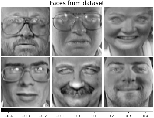
讓我們看一下我們的資料。灰色表示負值，白色表示正值。

plot_gallery("Faces from dataset", faces_centered[:n_components])

分解#

初始化不同的分解估計器，並將它們分別擬合到所有圖像上，並繪製一些結果。每個估計器都提取 6 個組件作為向量 \(h \in \mathbb{R}^{4096}\)。我們只是以方便人類理解的可視化方式，將這些向量顯示為 64x64 像素的圖像。

在使用者指南中閱讀更多資訊。

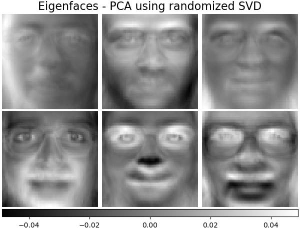
特徵臉 - 使用隨機 SVD 的 PCA#

使用資料的奇異值分解 (SVD) 進行線性降維，將其投影到較低的維度空間。

注意

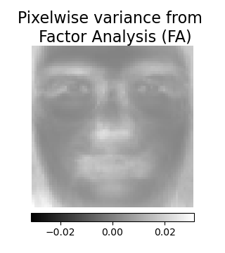
特徵臉估計器透過 sklearn.decomposition.PCA，還提供一個純量 noise_variance_（像素方向變異數的平均值），無法顯示為圖像。

pca_estimator = decomposition.PCA(
    n_components=n_components, svd_solver="randomized", whiten=True
)
pca_estimator.fit(faces_centered)
plot_gallery(
    "Eigenfaces - PCA using randomized SVD", pca_estimator.components_[:n_components]
)

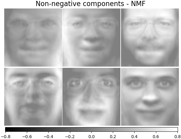
非負組件 - NMF#

估計非負原始資料作為兩個非負矩陣的乘積。

nmf_estimator = decomposition.NMF(n_components=n_components, tol=5e-3)
nmf_estimator.fit(faces)  # original non- negative dataset
plot_gallery("Non-negative components - NMF", nmf_estimator.components_[:n_components])

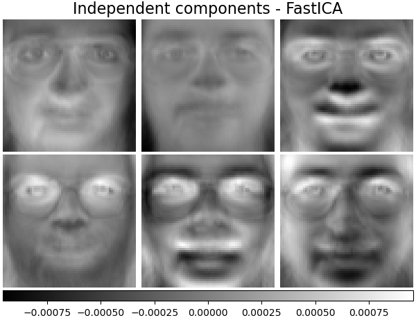
獨立組件 - FastICA#

獨立成分分析將多變量向量分解為彼此最大獨立的加性子成分。

ica_estimator = decomposition.FastICA(
    n_components=n_components, max_iter=400, whiten="arbitrary-variance", tol=15e-5
)
ica_estimator.fit(faces_centered)
plot_gallery(
    "Independent components - FastICA", ica_estimator.components_[:n_components]
)

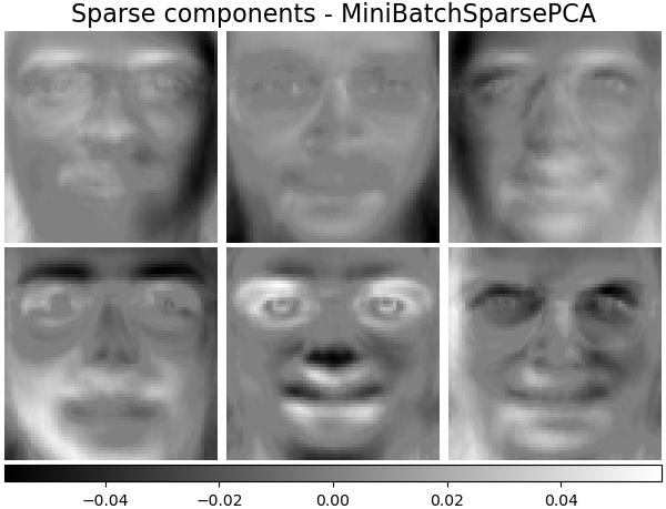
稀疏組件 - MiniBatchSparsePCA#

小批量稀疏 PCA (MiniBatchSparsePCA) 提取最能重建資料的一組稀疏組件。此變體比類似的 SparsePCA更快，但準確度較低。

batch_pca_estimator = decomposition.MiniBatchSparsePCA(
    n_components=n_components, alpha=0.1, max_iter=100, batch_size=3, random_state=rng
)
batch_pca_estimator.fit(faces_centered)
plot_gallery(
    "Sparse components - MiniBatchSparsePCA",
    batch_pca_estimator.components_[:n_components],
)

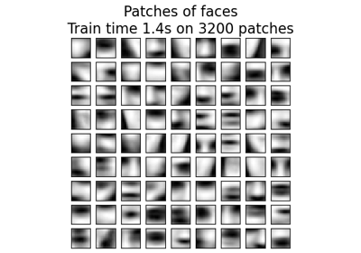
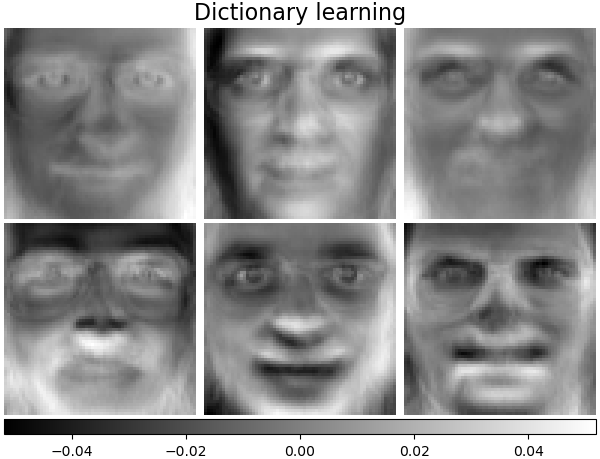
字典學習#

預設情況下，MiniBatchDictionaryLearning 將資料分成小批量，並透過在指定次數的迭代中循環小批量，以線上方式進行最佳化。

batch_dict_estimator = decomposition.MiniBatchDictionaryLearning(
    n_components=n_components, alpha=0.1, max_iter=50, batch_size=3, random_state=rng
)
batch_dict_estimator.fit(faces_centered)
plot_gallery("Dictionary learning", batch_dict_estimator.components_[:n_components])

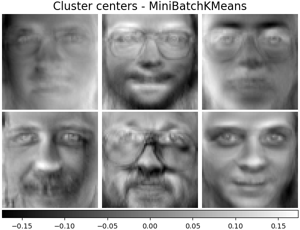
叢集中心 - MiniBatchKMeans#

sklearn.cluster.MiniBatchKMeans 在計算上是有效率的，並使用 partial_fit 方法實作線上學習。這就是為什麼用 MiniBatchKMeans 來增強一些耗時的演算法可能是有益的。

kmeans_estimator = cluster.MiniBatchKMeans(
    n_clusters=n_components,
    tol=1e-3,
    batch_size=20,
    max_iter=50,
    random_state=rng,
)
kmeans_estimator.fit(faces_centered)
plot_gallery(
    "Cluster centers - MiniBatchKMeans",
    kmeans_estimator.cluster_centers_[:n_components],
)

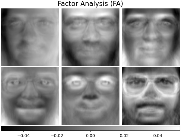
因子分析組件 - FA#

FactorAnalysis 與 PCA 相似，但具有獨立地對輸入空間每個方向的變異數進行建模的優點（異質雜訊）。在使用者指南中閱讀更多資訊。

fa_estimator = decomposition.FactorAnalysis(n_components=n_components, max_iter=20)
fa_estimator.fit(faces_centered)
plot_gallery("Factor Analysis (FA)", fa_estimator.components_[:n_components])

# --- Pixelwise variance
plt.figure(figsize=(3.2, 3.6), facecolor="white", tight_layout=True)
vec = fa_estimator.noise_variance_
vmax = max(vec.max(), -vec.min())
plt.imshow(
    vec.reshape(image_shape),
    cmap=plt.cm.gray,
    interpolation="nearest",
    vmin=-vmax,
    vmax=vmax,
)
plt.axis("off")
plt.title("Pixelwise variance from \n Factor Analysis (FA)", size=16, wrap=True)
plt.colorbar(orientation="horizontal", shrink=0.8, pad=0.03)
plt.show()

分解：字典學習#

在接下來的章節中，讓我們更精確地考慮字典學習。字典學習是一個問題，它相當於找到輸入資料的稀疏表示，作為簡單元素的組合。這些簡單元素構成一個字典。可以限制字典和/或編碼係數為正值，以符合資料中可能存在的限制。

MiniBatchDictionaryLearning 實作了字典學習演算法的更快但準確度較低的變體，更適合大型資料集。在使用者指南中閱讀更多資訊。

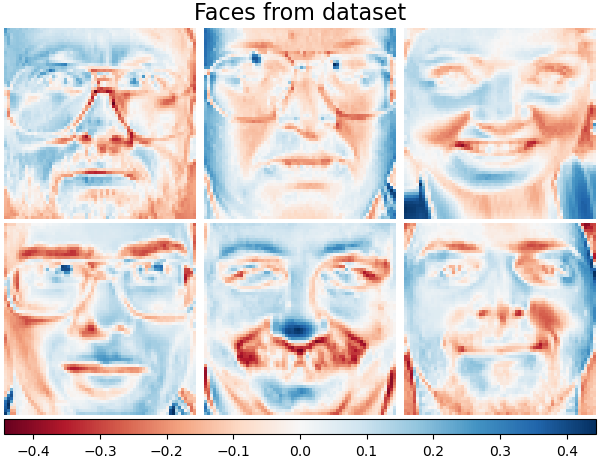
使用另一個顏色圖繪製我們資料集中相同的樣本。紅色表示負值，藍色表示正值，白色表示零。

plot_gallery("Faces from dataset", faces_centered[:n_components], cmap=plt.cm.RdBu)

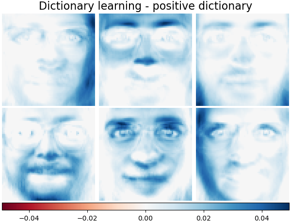
與先前的範例類似，我們更改參數並在所有圖像上訓練 MiniBatchDictionaryLearning 估計器。一般來說，字典學習和稀疏編碼會將輸入資料分解為字典和編碼係數矩陣。\(X \approx UV\)，其中 \(X = [x_1, . . . , x_n]\), \(X \in \mathbb{R}^{m×n}\)、字典 \(U \in \mathbb{R}^{m×k}\)、編碼係數 \(V \in \mathbb{R}^{k×n}\)。

以下是字典和編碼係數受到正向約束時的結果。

字典學習 - 正向字典#

在以下章節中，我們在尋找字典時強制執行正向性。

dict_pos_dict_estimator = decomposition.MiniBatchDictionaryLearning(
    n_components=n_components,
    alpha=0.1,
    max_iter=50,
    batch_size=3,
    random_state=rng,
    positive_dict=True,
)
dict_pos_dict_estimator.fit(faces_centered)
plot_gallery(
    "Dictionary learning - positive dictionary",
    dict_pos_dict_estimator.components_[:n_components],
    cmap=plt.cm.RdBu,
)

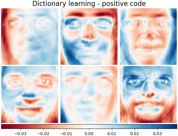
Dictionary learning - positive dictionary

字典學習 - 正向編碼#

以下我們將編碼係數限制為正矩陣。

dict_pos_code_estimator = decomposition.MiniBatchDictionaryLearning(
    n_components=n_components,
    alpha=0.1,
    max_iter=50,
    batch_size=3,
    fit_algorithm="cd",
    random_state=rng,
    positive_code=True,
)
dict_pos_code_estimator.fit(faces_centered)
plot_gallery(
    "Dictionary learning - positive code",
    dict_pos_code_estimator.components_[:n_components],
    cmap=plt.cm.RdBu,
)

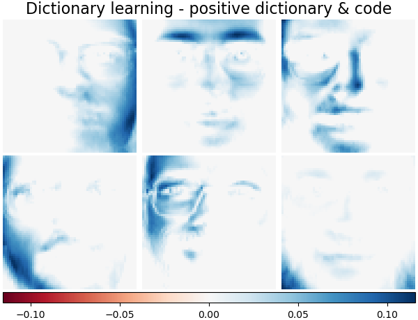
字典學習 - 正向字典和編碼#

以下是字典值和編碼係數受到正向約束時的結果。

dict_pos_estimator = decomposition.MiniBatchDictionaryLearning(
    n_components=n_components,
    alpha=0.1,
    max_iter=50,
    batch_size=3,
    fit_algorithm="cd",
    random_state=rng,
    positive_dict=True,
    positive_code=True,
)
dict_pos_estimator.fit(faces_centered)
plot_gallery(
    "Dictionary learning - positive dictionary & code",
    dict_pos_estimator.components_[:n_components],
    cmap=plt.cm.RdBu,
)