使用成本複雜性剪枝對決策樹進行後剪枝#

DecisionTreeClassifier 提供了諸如 min_samples_leaf 和 max_depth 等參數，以防止樹過擬合。成本複雜性剪枝提供了另一種控制樹大小的選項。在 DecisionTreeClassifier 中，此剪枝技術由成本複雜性參數 ccp_alpha 參數化。ccp_alpha 的值越大，修剪的節點數越多。這裡我們只展示 ccp_alpha 對正規化樹的影響，以及如何根據驗證分數選擇 ccp_alpha。

另請參閱最小成本複雜性剪枝以取得有關剪枝的詳細資訊。

# Authors: The scikit-learn developers
# SPDX-License-Identifier: BSD-3-Clause

import matplotlib.pyplot as plt

from sklearn.datasets import load_breast_cancer
from sklearn.model_selection import train_test_split
from sklearn.tree import DecisionTreeClassifier

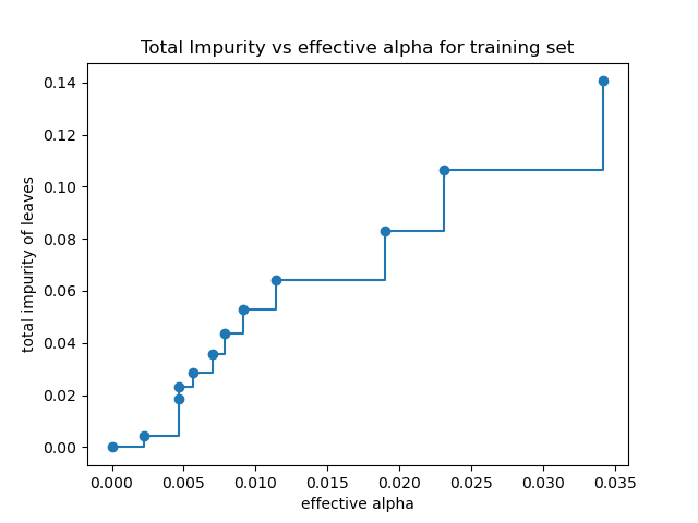
葉子的總雜質與修剪樹的有效 alpha 值#

最小成本複雜性剪枝會遞迴尋找具有「最弱連結」的節點。最弱連結的特徵在於有效 alpha 值，其中具有最小有效 alpha 值的節點會先被修剪。為了了解 ccp_alpha 的哪些值可能適用，scikit-learn 提供了 DecisionTreeClassifier.cost_complexity_pruning_path，它會傳回有效 alpha 值以及剪枝過程中每個步驟的對應葉子總雜質。隨著 alpha 增加，會修剪樹的更多部分，這會增加其葉子的總雜質。

X, y = load_breast_cancer(return_X_y=True)
X_train, X_test, y_train, y_test = train_test_split(X, y, random_state=0)

clf = DecisionTreeClassifier(random_state=0)
path = clf.cost_complexity_pruning_path(X_train, y_train)
ccp_alphas, impurities = path.ccp_alphas, path.impurities

在下圖中，已移除最大有效 alpha 值，因為它是只有一個節點的平凡樹。

fig, ax = plt.subplots()
ax.plot(ccp_alphas[:-1], impurities[:-1], marker="o", drawstyle="steps-post")
ax.set_xlabel("effective alpha")
ax.set_ylabel("total impurity of leaves")
ax.set_title("Total Impurity vs effective alpha for training set")

Total Impurity vs effective alpha for training set

Text(0.5, 1.0, 'Total Impurity vs effective alpha for training set')

接下來，我們使用有效 alpha 值訓練決策樹。ccp_alphas 中的最後一個值是修剪整個樹的 alpha 值，使樹 clfs[-1] 剩餘一個節點。

clfs = []
for ccp_alpha in ccp_alphas:
    clf = DecisionTreeClassifier(random_state=0, ccp_alpha=ccp_alpha)
    clf.fit(X_train, y_train)
    clfs.append(clf)
print(
    "Number of nodes in the last tree is: {} with ccp_alpha: {}".format(
        clfs[-1].tree_.node_count, ccp_alphas[-1]
    )
)

Number of nodes in the last tree is: 1 with ccp_alpha: 0.3272984419327777

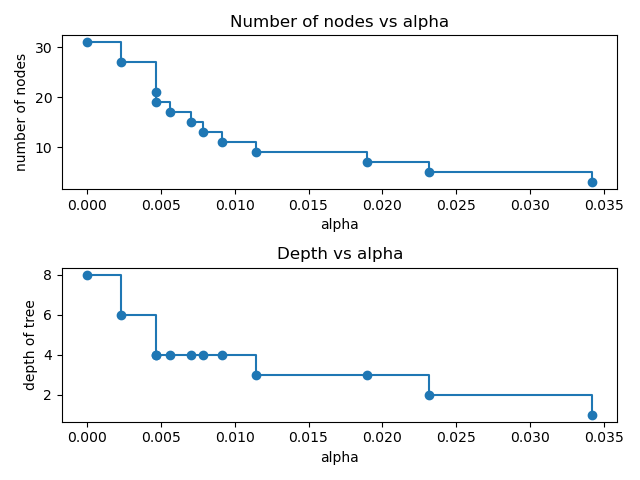
在本範例的其餘部分，我們移除 clfs 和 ccp_alphas 中的最後一個元素，因為它是只有一個節點的平凡樹。這裡我們展示節點數量和樹深度如何隨著 alpha 增加而減少。

clfs = clfs[:-1]
ccp_alphas = ccp_alphas[:-1]

node_counts = [clf.tree_.node_count for clf in clfs]
depth = [clf.tree_.max_depth for clf in clfs]
fig, ax = plt.subplots(2, 1)
ax[0].plot(ccp_alphas, node_counts, marker="o", drawstyle="steps-post")
ax[0].set_xlabel("alpha")
ax[0].set_ylabel("number of nodes")
ax[0].set_title("Number of nodes vs alpha")
ax[1].plot(ccp_alphas, depth, marker="o", drawstyle="steps-post")
ax[1].set_xlabel("alpha")
ax[1].set_ylabel("depth of tree")
ax[1].set_title("Depth vs alpha")
fig.tight_layout()

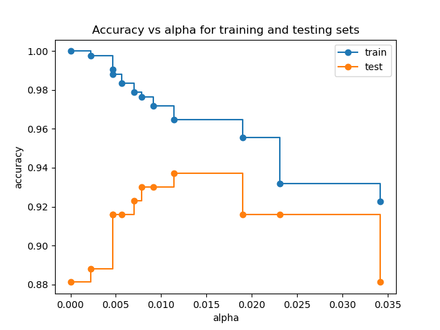
Number of nodes vs alpha, Depth vs alpha

訓練和測試集的準確度與 alpha 值#

當 ccp_alpha 設定為零並保持 DecisionTreeClassifier 的其他預設參數時，樹會過擬合，導致 100% 的訓練準確度和 88% 的測試準確度。隨著 alpha 增加，樹的更多部分會被修剪，因此會建立一個泛化效果更好的決策樹。在本範例中，設定 ccp_alpha=0.015 可以最大化測試準確度。

train_scores = [clf.score(X_train, y_train) for clf in clfs]
test_scores = [clf.score(X_test, y_test) for clf in clfs]

fig, ax = plt.subplots()
ax.set_xlabel("alpha")
ax.set_ylabel("accuracy")
ax.set_title("Accuracy vs alpha for training and testing sets")
ax.plot(ccp_alphas, train_scores, marker="o", label="train", drawstyle="steps-post")
ax.plot(ccp_alphas, test_scores, marker="o", label="test", drawstyle="steps-post")
ax.legend()
plt.show()