單一估計器與裝袋：偏差-變異分解#

此範例說明並比較單一估計器與裝袋集成預期均方誤差的偏差-變異分解。

在迴歸中，估計器的預期均方誤差可以分解為偏差、變異數和雜訊。在迴歸問題的資料集平均值上，偏差項衡量估計器的預測與問題最佳可能估計器（即貝氏模型）預測之間的平均差異量。變異項衡量估計器在針對相同問題的不同隨機實例進行擬合時預測的變異性。在以下內容中，每個問題實例都以「LS」表示，代表「學習樣本」。最後，雜訊衡量的是由於資料變異性而導致的不可簡化誤差部分。

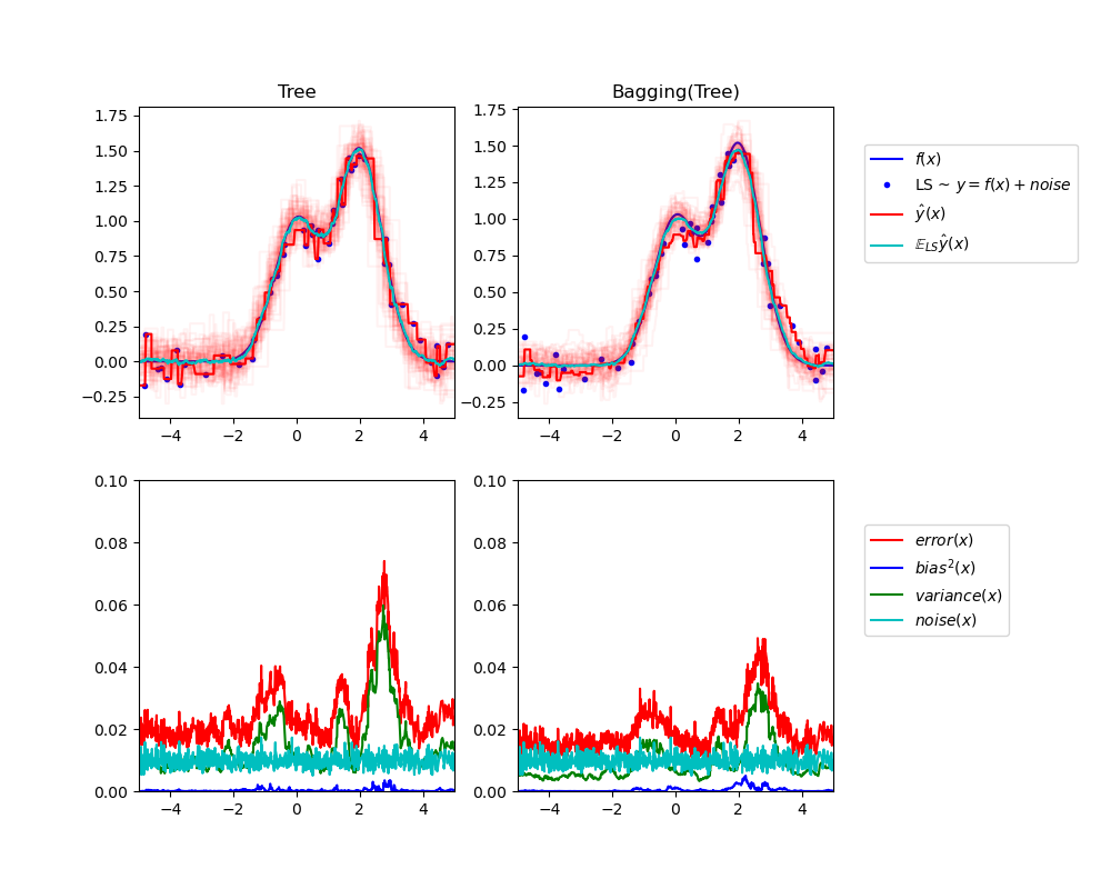
左上圖說明了在玩具 1d 迴歸問題的隨機資料集 LS（藍色點）上訓練的單一決策樹的預測（深紅色）。它也說明了在問題的其他（和不同）隨機繪製的 LS 實例上訓練的其他單一決策樹的預測（淺紅色）。直觀地說，此處的變異項對應於個別估計器的預測（淺紅色）的光束寬度。變異數越大，x 的預測就越容易受到訓練集中微小變化的影響。偏差項對應於估計器的平均預測（青色）與最佳可能模型（深藍色）之間的差異。因此，在這個問題中，我們可以觀察到偏差相當低（青色曲線和藍色曲線彼此接近），而變異數很大（紅色光束相當寬）。

左下圖繪製了單一決策樹預期均方誤差的逐點分解。它證實了偏差項（藍色）較低，而變異數較大（綠色）。它也說明了誤差的雜訊部分，如預期的那樣，它看起來是恆定的且約為 0.01。

右側的圖表對應於相同的圖表，但改為使用決策樹的裝袋集成。在這兩個圖表中，我們都可以觀察到偏差項比前一種情況更大。在右上圖中，平均預測（青色）與最佳可能模型之間的差異更大（例如，請注意 x=2 附近的偏移）。在右下圖中，偏差曲線也略高於左下圖。然而，就變異數而言，預測光束更窄，這表示變異數較低。事實上，正如右下圖所證實的，變異項（綠色）低於單一決策樹。整體而言，因此偏差-變異分解不再相同。裝袋的權衡更好：平均多個在資料集的引導副本上擬合的決策樹會稍微增加偏差項，但允許更大程度地降低變異數，從而導致較低的整體均方誤差（比較下圖中的紅色曲線）。腳本輸出也證實了這種直覺。裝袋集成的總誤差低於單一決策樹的總誤差，而這種差異實際上主要來自降低的變異數。

有關偏差-變異分解的更多詳細資訊，請參閱 [1] 的 7.3 節。

參考文獻#

Tree: 0.0255 (error) = 0.0003 (bias^2)  + 0.0152 (var) + 0.0098 (noise)
Bagging(Tree): 0.0196 (error) = 0.0004 (bias^2)  + 0.0092 (var) + 0.0098 (noise)

# Authors: The scikit-learn developers
# SPDX-License-Identifier: BSD-3-Clause

import matplotlib.pyplot as plt
import numpy as np

from sklearn.ensemble import BaggingRegressor
from sklearn.tree import DecisionTreeRegressor

# Settings
n_repeat = 50  # Number of iterations for computing expectations
n_train = 50  # Size of the training set
n_test = 1000  # Size of the test set
noise = 0.1  # Standard deviation of the noise
np.random.seed(0)

# Change this for exploring the bias-variance decomposition of other
# estimators. This should work well for estimators with high variance (e.g.,
# decision trees or KNN), but poorly for estimators with low variance (e.g.,
# linear models).
estimators = [
    ("Tree", DecisionTreeRegressor()),
    ("Bagging(Tree)", BaggingRegressor(DecisionTreeRegressor())),
]

n_estimators = len(estimators)


# Generate data
def f(x):
    x = x.ravel()

    return np.exp(-(x**2)) + 1.5 * np.exp(-((x - 2) ** 2))


def generate(n_samples, noise, n_repeat=1):
    X = np.random.rand(n_samples) * 10 - 5
    X = np.sort(X)

    if n_repeat == 1:
        y = f(X) + np.random.normal(0.0, noise, n_samples)
    else:
        y = np.zeros((n_samples, n_repeat))

        for i in range(n_repeat):
            y[:, i] = f(X) + np.random.normal(0.0, noise, n_samples)

    X = X.reshape((n_samples, 1))

    return X, y


X_train = []
y_train = []

for i in range(n_repeat):
    X, y = generate(n_samples=n_train, noise=noise)
    X_train.append(X)
    y_train.append(y)

X_test, y_test = generate(n_samples=n_test, noise=noise, n_repeat=n_repeat)

plt.figure(figsize=(10, 8))

# Loop over estimators to compare
for n, (name, estimator) in enumerate(estimators):
    # Compute predictions
    y_predict = np.zeros((n_test, n_repeat))

    for i in range(n_repeat):
        estimator.fit(X_train[i], y_train[i])
        y_predict[:, i] = estimator.predict(X_test)

    # Bias^2 + Variance + Noise decomposition of the mean squared error
    y_error = np.zeros(n_test)

    for i in range(n_repeat):
        for j in range(n_repeat):
            y_error += (y_test[:, j] - y_predict[:, i]) ** 2

    y_error /= n_repeat * n_repeat

    y_noise = np.var(y_test, axis=1)
    y_bias = (f(X_test) - np.mean(y_predict, axis=1)) ** 2
    y_var = np.var(y_predict, axis=1)

    print(
        "{0}: {1:.4f} (error) = {2:.4f} (bias^2) "
        " + {3:.4f} (var) + {4:.4f} (noise)".format(
            name, np.mean(y_error), np.mean(y_bias), np.mean(y_var), np.mean(y_noise)
        )
    )

    # Plot figures
    plt.subplot(2, n_estimators, n + 1)
    plt.plot(X_test, f(X_test), "b", label="$f(x)$")
    plt.plot(X_train[0], y_train[0], ".b", label="LS ~ $y = f(x)+noise$")

    for i in range(n_repeat):
        if i == 0:
            plt.plot(X_test, y_predict[:, i], "r", label=r"$\^y(x)$")
        else:
            plt.plot(X_test, y_predict[:, i], "r", alpha=0.05)

    plt.plot(X_test, np.mean(y_predict, axis=1), "c", label=r"$\mathbb{E}_{LS} \^y(x)$")

    plt.xlim([-5, 5])
    plt.title(name)

    if n == n_estimators - 1:
        plt.legend(loc=(1.1, 0.5))

    plt.subplot(2, n_estimators, n_estimators + n + 1)
    plt.plot(X_test, y_error, "r", label="$error(x)$")
    plt.plot(X_test, y_bias, "b", label="$bias^2(x)$"),
    plt.plot(X_test, y_var, "g", label="$variance(x)$"),
    plt.plot(X_test, y_noise, "c", label="$noise(x)$")

    plt.xlim([-5, 5])
    plt.ylim([0, 0.1])

    if n == n_estimators - 1:
        plt.legend(loc=(1.1, 0.5))

plt.subplots_adjust(right=0.75)
plt.show()