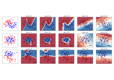
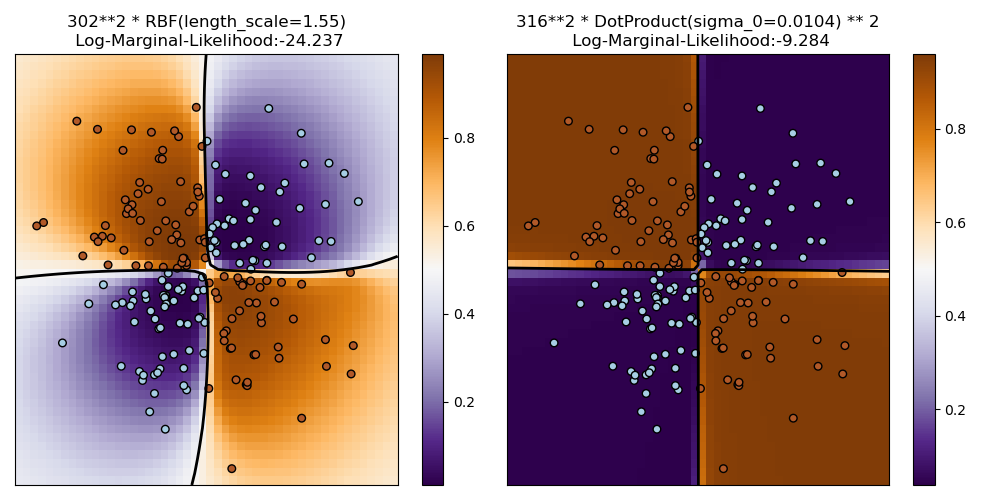
XOR 資料集上的高斯過程分類 (GPC) 說明#

此範例說明 XOR 資料上的 GPC。比較的是一個靜態、等向性核 (RBF) 和一個非靜態核 (DotProduct)。在這個特定的資料集上，DotProduct 核獲得了明顯更好的結果，因為類別邊界是線性的，並且與座標軸重合。一般來說，靜態核通常會獲得更好的結果。

302**2 * RBF(length_scale=1.55) Log-Marginal-Likelihood:-24.237, 316**2 * DotProduct(sigma_0=0.0104) ** 2 Log-Marginal-Likelihood:-9.284

/home/circleci/project/sklearn/gaussian_process/kernels.py:452: ConvergenceWarning:

The optimal value found for dimension 0 of parameter k1__constant_value is close to the specified upper bound 100000.0. Increasing the bound and calling fit again may find a better value.

# Authors: The scikit-learn developers
# SPDX-License-Identifier: BSD-3-Clause

import matplotlib.pyplot as plt
import numpy as np

from sklearn.gaussian_process import GaussianProcessClassifier
from sklearn.gaussian_process.kernels import RBF, DotProduct

xx, yy = np.meshgrid(np.linspace(-3, 3, 50), np.linspace(-3, 3, 50))
rng = np.random.RandomState(0)
X = rng.randn(200, 2)
Y = np.logical_xor(X[:, 0] > 0, X[:, 1] > 0)

# fit the model
plt.figure(figsize=(10, 5))
kernels = [1.0 * RBF(length_scale=1.15), 1.0 * DotProduct(sigma_0=1.0) ** 2]
for i, kernel in enumerate(kernels):
    clf = GaussianProcessClassifier(kernel=kernel, warm_start=True).fit(X, Y)

    # plot the decision function for each datapoint on the grid
    Z = clf.predict_proba(np.vstack((xx.ravel(), yy.ravel())).T)[:, 1]
    Z = Z.reshape(xx.shape)

    plt.subplot(1, 2, i + 1)
    image = plt.imshow(
        Z,
        interpolation="nearest",
        extent=(xx.min(), xx.max(), yy.min(), yy.max()),
        aspect="auto",
        origin="lower",
        cmap=plt.cm.PuOr_r,
    )
    contours = plt.contour(xx, yy, Z, levels=[0.5], linewidths=2, colors=["k"])
    plt.scatter(X[:, 0], X[:, 1], s=30, c=Y, cmap=plt.cm.Paired, edgecolors=(0, 0, 0))
    plt.xticks(())
    plt.yticks(())
    plt.axis([-3, 3, -3, 3])
    plt.colorbar(image)
    plt.title(
        "%s\n Log-Marginal-Likelihood:%.3f"
        % (clf.kernel_, clf.log_marginal_likelihood(clf.kernel_.theta)),
        fontsize=12,
    )

plt.tight_layout()
plt.show()