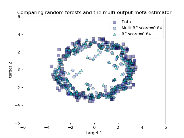
比較隨機森林和多輸出元估計器#

一個比較隨機森林和 multioutput.MultiOutputRegressor 元估計器的多輸出迴歸的範例。

此範例說明如何使用 multioutput.MultiOutputRegressor 元估計器執行多輸出迴歸。使用原生支援多輸出迴歸的隨機森林迴歸器，因此可以比較結果。

隨機森林迴歸器只會預測在每個目標的觀察範圍內或更接近零的值。因此，預測會偏向圓的中心。

使用單個底層特徵，模型會將 x 和 y 坐標都作為輸出學習。

Comparing random forests and the multi-output meta estimator

# Authors: The scikit-learn developers
# SPDX-License-Identifier: BSD-3-Clause

import matplotlib.pyplot as plt
import numpy as np

from sklearn.ensemble import RandomForestRegressor
from sklearn.model_selection import train_test_split
from sklearn.multioutput import MultiOutputRegressor

# Create a random dataset
rng = np.random.RandomState(1)
X = np.sort(200 * rng.rand(600, 1) - 100, axis=0)
y = np.array([np.pi * np.sin(X).ravel(), np.pi * np.cos(X).ravel()]).T
y += 0.5 - rng.rand(*y.shape)

X_train, X_test, y_train, y_test = train_test_split(
    X, y, train_size=400, test_size=200, random_state=4
)

max_depth = 30
regr_multirf = MultiOutputRegressor(
    RandomForestRegressor(n_estimators=100, max_depth=max_depth, random_state=0)
)
regr_multirf.fit(X_train, y_train)

regr_rf = RandomForestRegressor(n_estimators=100, max_depth=max_depth, random_state=2)
regr_rf.fit(X_train, y_train)

# Predict on new data
y_multirf = regr_multirf.predict(X_test)
y_rf = regr_rf.predict(X_test)

# Plot the results
plt.figure()
s = 50
a = 0.4
plt.scatter(
    y_test[:, 0],
    y_test[:, 1],
    edgecolor="k",
    c="navy",
    s=s,
    marker="s",
    alpha=a,
    label="Data",
)
plt.scatter(
    y_multirf[:, 0],
    y_multirf[:, 1],
    edgecolor="k",
    c="cornflowerblue",
    s=s,
    alpha=a,
    label="Multi RF score=%.2f" % regr_multirf.score(X_test, y_test),
)
plt.scatter(
    y_rf[:, 0],
    y_rf[:, 1],
    edgecolor="k",
    c="c",
    s=s,
    marker="^",
    alpha=a,
    label="RF score=%.2f" % regr_rf.score(X_test, y_test),
)
plt.xlim([-6, 6])
plt.ylim([-6, 6])
plt.xlabel("target 1")
plt.ylabel("target 2")
plt.title("Comparing random forests and the multi-output meta estimator")
plt.legend()
plt.show()