注意
跳至結尾以下載完整的範例程式碼。或透過 JupyterLite 或 Binder 在您的瀏覽器中執行此範例
單變數特徵選擇#
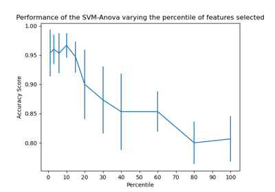
此筆記本是一個使用單變數特徵選擇來提高嘈雜資料集分類準確性的範例。
在此範例中,一些嘈雜(無資訊)特徵被添加到虹膜資料集中。支援向量機 (SVM) 用於在應用單變數特徵選擇之前和之後對資料集進行分類。對於每個特徵,我們繪製單變數特徵選擇的 p 值和相應的 SVM 權重。透過這種方式,我們將比較模型的準確性並檢視單變數特徵選擇對模型權重的影響。
# Authors: The scikit-learn developers
# SPDX-License-Identifier: BSD-3-Clause
產生範例資料#
import numpy as np

from sklearn.datasets import load_iris
from sklearn.model_selection import train_test_split

# The iris dataset
X, y = load_iris(return_X_y=True)

# Some noisy data not correlated
E = np.random.RandomState(42).uniform(0, 0.1, size=(X.shape[0], 20))

# Add the noisy data to the informative features
X = np.hstack((X, E))

# Split dataset to select feature and evaluate the classifier
X_train, X_test, y_train, y_test = train_test_split(X, y, stratify=y, random_state=0)
單變數特徵選擇#
使用 F 檢定進行特徵評分的單變數特徵選擇。我們使用預設選擇函數來選擇四個最重要的特徵。
from sklearn.feature_selection import SelectKBest, f_classif

selector = SelectKBest(f_classif, k=4)
selector.fit(X_train, y_train)
scores = -np.log10(selector.pvalues_)
scores /= scores.max()
import matplotlib.pyplot as plt

X_indices = np.arange(X.shape[-1])
plt.figure(1)
plt.clf()
plt.bar(X_indices - 0.05, scores, width=0.2)
plt.title("Feature univariate score")
plt.xlabel("Feature number")
plt.ylabel(r"Univariate score ($-Log(p_{value})$)")
plt.show()
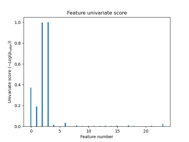
在所有特徵中,只有 4 個原始特徵是顯著的。我們可以發現它們在單變數特徵選擇中具有最高分數。
與 SVM 比較#
沒有單變數特徵選擇
from sklearn.pipeline import make_pipeline
from sklearn.preprocessing import MinMaxScaler
from sklearn.svm import LinearSVC

clf = make_pipeline(MinMaxScaler(), LinearSVC())
clf.fit(X_train, y_train)
print(
    "Classification accuracy without selecting features: {:.3f}".format(
        clf.score(X_test, y_test)
    )
)

svm_weights = np.abs(clf[-1].coef_).sum(axis=0)
svm_weights /= svm_weights.sum()
Classification accuracy without selecting features: 0.789
在單變數特徵選擇之後
clf_selected = make_pipeline(SelectKBest(f_classif, k=4), MinMaxScaler(), LinearSVC())
clf_selected.fit(X_train, y_train)
print(
    "Classification accuracy after univariate feature selection: {:.3f}".format(
        clf_selected.score(X_test, y_test)
    )
)

svm_weights_selected = np.abs(clf_selected[-1].coef_).sum(axis=0)
svm_weights_selected /= svm_weights_selected.sum()
Classification accuracy after univariate feature selection: 0.868
plt.bar(
    X_indices - 0.45, scores, width=0.2, label=r"Univariate score ($-Log(p_{value})$)"
)

plt.bar(X_indices - 0.25, svm_weights, width=0.2, label="SVM weight")

plt.bar(
    X_indices[selector.get_support()] - 0.05,
    svm_weights_selected,
    width=0.2,
    label="SVM weights after selection",
)

plt.title("Comparing feature selection")
plt.xlabel("Feature number")
plt.yticks(())
plt.axis("tight")
plt.legend(loc="upper right")
plt.show()
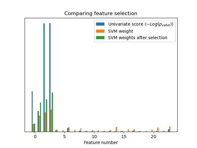
沒有單變數特徵選擇,SVM 會將較大的權重分配給前 4 個原始顯著特徵,但也會選擇許多無資訊的特徵。在 SVM 之前應用單變數特徵選擇會增加 SVM 歸因於顯著特徵的權重,因此將提高分類。
腳本的總執行時間: (0 分鐘 0.190 秒)
相關範例