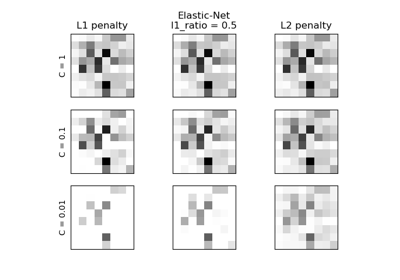
Lasso 和彈性網路#

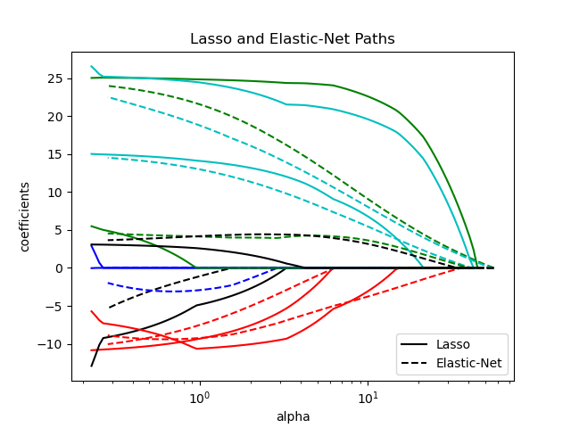
使用坐標下降法實現的 Lasso 和彈性網路（L1 和 L2 懲罰）。

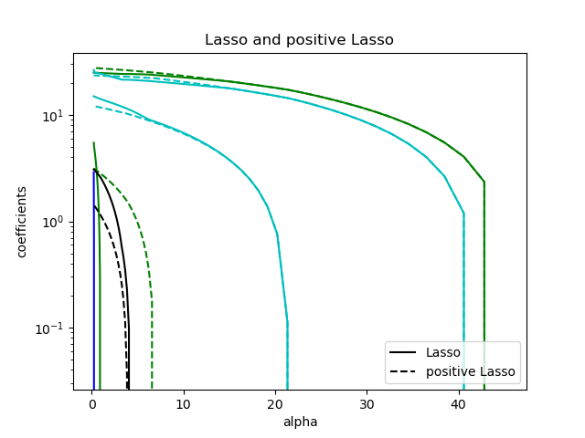
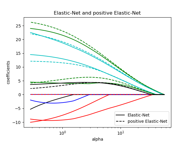
係數可以強制為正。

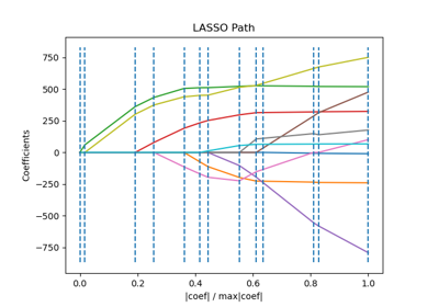
Computing regularization path using the lasso...
Computing regularization path using the positive lasso...
Computing regularization path using the elastic net...
Computing regularization path using the positive elastic net...

# Author: Alexandre Gramfort <alexandre.gramfort@inria.fr>
# License: BSD 3 clause

from itertools import cycle

import matplotlib.pyplot as plt

from sklearn import datasets
from sklearn.linear_model import enet_path, lasso_path

X, y = datasets.load_diabetes(return_X_y=True)


X /= X.std(axis=0)  # Standardize data (easier to set the l1_ratio parameter)

# Compute paths

eps = 5e-3  # the smaller it is the longer is the path

print("Computing regularization path using the lasso...")
alphas_lasso, coefs_lasso, _ = lasso_path(X, y, eps=eps)

print("Computing regularization path using the positive lasso...")
alphas_positive_lasso, coefs_positive_lasso, _ = lasso_path(
    X, y, eps=eps, positive=True
)
print("Computing regularization path using the elastic net...")
alphas_enet, coefs_enet, _ = enet_path(X, y, eps=eps, l1_ratio=0.8)

print("Computing regularization path using the positive elastic net...")
alphas_positive_enet, coefs_positive_enet, _ = enet_path(
    X, y, eps=eps, l1_ratio=0.8, positive=True
)

# Display results

plt.figure(1)
colors = cycle(["b", "r", "g", "c", "k"])
for coef_l, coef_e, c in zip(coefs_lasso, coefs_enet, colors):
    l1 = plt.semilogx(alphas_lasso, coef_l, c=c)
    l2 = plt.semilogx(alphas_enet, coef_e, linestyle="--", c=c)

plt.xlabel("alpha")
plt.ylabel("coefficients")
plt.title("Lasso and Elastic-Net Paths")
plt.legend((l1[-1], l2[-1]), ("Lasso", "Elastic-Net"), loc="lower right")
plt.axis("tight")


plt.figure(2)
for coef_l, coef_pl, c in zip(coefs_lasso, coefs_positive_lasso, colors):
    l1 = plt.semilogy(alphas_lasso, coef_l, c=c)
    l2 = plt.semilogy(alphas_positive_lasso, coef_pl, linestyle="--", c=c)

plt.xlabel("alpha")
plt.ylabel("coefficients")
plt.title("Lasso and positive Lasso")
plt.legend((l1[-1], l2[-1]), ("Lasso", "positive Lasso"), loc="lower right")
plt.axis("tight")


plt.figure(3)
for coef_e, coef_pe, c in zip(coefs_enet, coefs_positive_enet, colors):
    l1 = plt.semilogx(alphas_enet, coef_e, c=c)
    l2 = plt.semilogx(alphas_positive_enet, coef_pe, linestyle="--", c=c)

plt.xlabel("alpha")
plt.ylabel("coefficients")
plt.title("Elastic-Net and positive Elastic-Net")
plt.legend((l1[-1], l2[-1]), ("Elastic-Net", "positive Elastic-Net"), loc="lower right")
plt.axis("tight")
plt.show()